

Battle of the Pricing Models: Trees vs Monte Carlo
By Rich Tanenbaum, Savvysoft
I was having a conversation with a client the other day and the subject of Monte Carlo simulation and binomial trees came up. Often, people think of these as distinctly different methods to price derivatives. What they don’t always realize are some of the similarities between the two. I thought you might be interested in learning about it, too.
First, a little bit of background. A binomial tree model is based on building a structure of possible prices an asset can have over time. It looks like this:
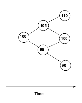
Each of the circles is a node, which represents a price of the underlying asset. The current price is on the far left, and the price can go either up or down over a given time period. As we move to the right, we’re moving forward through time. So there are two possible prices the asset can have after one period. In this tree, if it moves up in the first period, and moves down in the second period, it will be the same price as if it moves down in the first period and then moves up in the second period. This means there are only three possible prices after two periods. We call this a recombining tree. If an up move followed by a down move doesn’t lead to the same price as a down move followed by an up move, the tree would look like this:
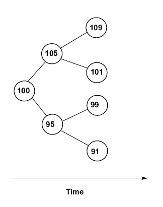
This is called a non-recombining, or bushy, tree. When calculating an option price using a tree model, calculations will be done in each node of the tree, so the more nodes you have, the longer it takes to run the model. This makes recombining trees far better than bushy ones. How much better? Well, if you have 30 time periods, then a recombining tree will have 240 nodes. But a bushy tree will have over two million nodes!
To price an option using a tree, we start by building the tree, going out to expiration. We then calculate the option value in each node at the end of the tree, the nodes on the far right. This is easy to do, given the strike and the price of the asset in each node. Then, in each node in the second to last time period, the option price is equal to present value of the average of the two option prices coming out that node. After the option prices have been calculated in each node in the second to last period, the same procedure can be followed to price the option in each node of the third to last period. This continues until we have a single option price in the first node, and we’re done.
That’s how European option pricing works. American options are priced in much the same way, with one extra wrinkle: in each node, after calculating the present value of the average of the next two nodes, we compare that to the value of exercising the option in that node. Whichever of the two is greater is the option value for that node. This makes pricing American and Bermudan options very simple.
Monte Carlo simulation follows a seemingly different process. Given today’s price for the underlying asset, a random number is generated. Then, the price of the asset is adjusted based on the random number. For example, the random number might represent the asset’s return over a month, like 5% or -3%. The new asset price is then calculated, and another random number is drawn for the return over the second month. This is repeated for each month in the option’s life, to get a possible asset price at expiration. This is then compared to the strike price to get the option value at expiration. The option value is stored as simulation path number 1, and the process is repeated for the first month, the second month and so on with a new set of random numbers, to get the option price for simulation path 2. This is done, over and over again, perhaps for thousands of simulation paths. Then, we take the average of all the option prices, and present value the average back to today. This is the Monte Carlo value of the option.
Since the random numbers are, well, random, if we price the option this way twice we will get two different answers (unless the random numbers always start off the same way each time). This means that the price we get is a best guess, but subject to a range, plus or minus a bit, around that average. If we take the standard deviation of all the option prices in a run, and divide that by the square root of the number of simulations run, we get the standard error of the simulation run. The standard error is the amount of uncertainty around the average price, that plus or minus a bit. The more simulation paths we run, the smaller the standard error.
That’s how to price European options with a Monte Carlo simulation. To price American or Bermudan options, you…, well, it’s not that easy to do. There are ways that have been proposed, which give a biased estimate that is an estimate of an estimate, but it’s beyond the scope of this article to explain it, unlike the simplicity of handling it with a tree.
So besides being used to solve the same problem, how are trees and Monte Carlo alike? Quite simply, you can run a simulation by walking forwards through a tree. Start at the beginning of the tree, and make the random number be the result of a coin flip: heads and the price goes up, tails and the price goes down. Then flip the coin again to see if the price goes up or down in the next period. Flip it again for the next period, and so on, until you get to the end of the tree (the option’s expiration). Treat that as the first simulation path, and calculate the option value for that path. Then, go back to the beginning and do it all over again, just like in the Monte Carlo simulation described above. Do that a few thousand times, average the results, present value the average, and that’s the option value.
How does this compare to a real Monte Carlo simulation? It *is* a real Monte Carlo simulation. There are no rules about how the random numbers are generated, so using coin flips is just as valid as any other method. Some proponents of Monte Carlo will argue that a simulation can draw from a continuous distribution, where any type of number can be pulled out of a generator: 3.456843, or -4.4736364 or 6.484773 or anything else, rather than the simple and limited up and down from the tree. That is true, but if we have a decent number of time steps in the tree, the number of possible prices at the end of the tree is also large enough, and there are many more than just two possible prices. In effect, by breaking the life of the option into many time steps, there’s time for the underlying asset to take on many values at expiration.
It’s also true that, for European options, a Monte Carlo simulation doesn’t need to generate, say, twelve monthly returns for a one year option. Instead, one annual return, obtained from one random number, can be used to get the price of the underlying at expiration for each path. So for 10,000 paths, only 10,000 random numbers need to be drawn, and 10,000 intrinsic values need to be calculated. This would seem to allow Monte Carlo simulations to run quickly compared to trees.
But that would be misleading. First, this is only true for European options. And when a tree is used to price European options, the nodes before expiration can be skipped, too, thus requiring much fewer nodes and calculations. But in addition to all that, the Monte Carlo only gives an estimate, with a standard error attached to it.
The question is: how big is the standard error? That depends on the option and the number of simulation paths, of course. But whatever it is, I contend that the error in the tree, for any given option, is always smaller than the error in Monte Carlo.
To understand why, we have to talk about where the Monte Carlo error comes from in the first place. As noted above, two consecutive Monte Carlo runs will yield two different option values, unless the same random numbers are generated each time. This is because the random numbers are a sample of a distribution, and are therefore a subset which is meant to be representative of the whole, but is not a perfect match for the whole. In other words, the average of the random numbers we are looking for may be 0, but the first time it may come out to be 1%, and the second time it may come out to be -.5%. Likewise, we may ask the random number generator to give us numbers with a standard deviation of 20%, but the numbers that actually come back, may have a standard deviation of 21% due to random chance. So the random numbers are going to be a little biased, after the fact, sometimes one way, sometimes another way. And that causes the option value to be a little biased, sometimes one way, and sometimes the other way.
But the tree, when it is looked at like a Monte Carlo simulation, but used in the standard tree way by walking backwards, has exactly one path for every possibility. Taking the average of the up and down nodes to get the value in a prior node is the same as averaging two simulation paths, one that went up, and one that went down. If you look at the shortcut version of the binomial formula for European options (you’ll have to look for example at Cox Ross and Rubinstein’s paper for this), you see that the weight applied to each node at expiration is the probability of reaching that node; no more, and no less. So we use the precise random distribution of returns to price the option. It is as if we are running the simulation with one and only one path through the tree for each possibility. So the tree is like a perfect simulation that matches the distribution exactly. And this exact match means we don’t have the standard error that we get with a Monte Carlo simulation.
True, the Monte Carlo standard error gets smaller as more simulations are run. But let’s look at the numbers. As we said before, a non-recombining tree with 30 periods will have over two million nodes. This turns out to be the same number of distinct paths there are through a 30 period recombining tree, as both are 2^30. So the relatively small binomial tree is looking at as many possible paths as a two million path simulation. And, it’s hitting the distribution more precisely, making it much faster (over 4,000 times faster), and more accurate, than Monte Carlo.
That’s not to say that Monte Carlo simulation offers no advantages to trees. There are two examples worth stating:
1. Monte Carlo can be used for any type of distribution, including changing distributions. This means you’re not limited to normal or lognormal returns, and you can change distributional parameters like volatility. Some of this is also possible with a tree, but it’s more limited. For example, it may lead to a bushy tree.
2. Path dependent structures like lookbacks and Asian options are simpler to do with Monte Carlo simulation. Again, methods are available to handle these with trees too, but it seems more straightforward with Monte Carlo simulation.
It’s not clear how much value there is to choosing other distributions. While markets may not be perfectly lognormal, the extra value gained from using other models may be lost when one is forced to come up with the unobservable parameters to plug into the model. In other words, if you have some type of model that includes a volatility, but also some mean reversion factor, and you can’t see the mean reversion factor, then the simulation result won’t be reliable (garbage in, garbage out).
All that said, we do offer pricing models in TOPS and OmniPricer which employ Monte Carlo simulation, because we believe in using the right tool for the right job (if you'd like to give TOPS a try, for free, click here). But it’s also important to know how to choose the right tool, and the notion that a tree can be viewed as a perfect Monte Carlo simulation can help with that decision.